Amazon reviews
Hadoop for Amazon product co-purchasing network
Introduction
Sampling networks is not an easy and fast procedure. Consider taking samples from data sources like Amazon where hundreds of millions users and products are related. Any attempt to analyze the data without direct access is complicated. First, you would have to index semi-structured data in the form of HTML code, Amazon website, to get products and user. Once you have that information you would have to find a way to connect users. One additional problem is that products may not have a significant amount of ratings from where to build users networks, and it may yield sparse clouds and a large amount of time to sample with more data.
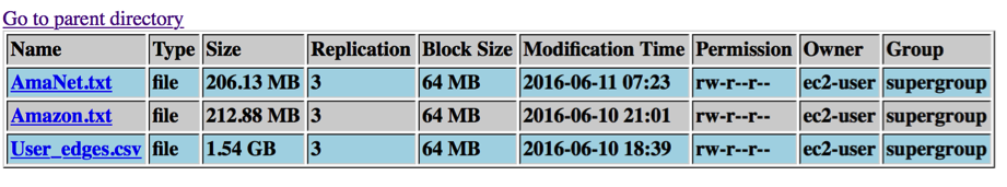
Using meta-data collected from Stanford University I would create samples to be analyzed. The data is about products sold on Amazon during the summer of 2006. The features for each product are title, sales rank, list of similar products, categories associated with the product and reviews including individual ratings from users. The products are books, DVDs, Music CDs and videos.
For sake of comparison, I have used python code to create samples using a simple Apple computer. The time to process a block of 100 thousand products (about 40 MB size) is around 5 hours to complete. The resulting network has over 15 million edges. In terms hard disk memory the sample uses 1.54 GB. I have also used single node server for this part and even when the time is reduced it requires many hours to complete using the same python code. Hadoop is helpful building the network, the edges and nodes do not need to be in the same physical space, I can process chunks of data and the put the resulting network together.
The Cluster
To process the data I set up a cluster using Amazon Cloud Services consisting of 3 medium size nodes with 20GB of volume for each node. HDFS replication factor is set to 3 as it is a simple small cluster for this exercise. Memory specification was modified since the reducer was running out of memory when creating the list of edges. Two additional properties are added. One of them sets more reducers by default when running Hadoop, and the second is the memory assign to each reducer.
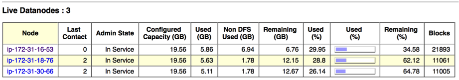
The nodes are somehow balanced in terms of the load that each one of them received during the project. Later we will see how HDFS is making a good job by itself keeping the cluster balanced.
Figure 1
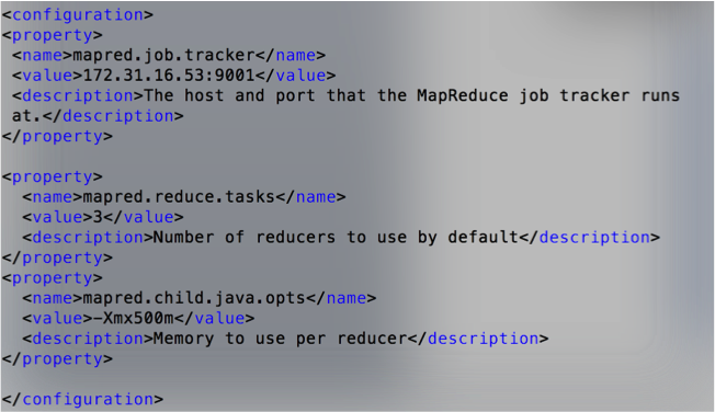
Figure 2
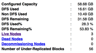
Figure 3
Loading data with Hive and PIG
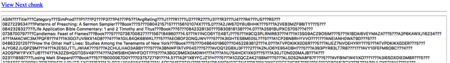
The raw data is semi-structured, the same I used for the a previous analysis on the Amazon data, when I process that data I also prepare some data for this analysis. However, the data was stored as texts files. For this project, a single file with all the nodes is created.
Figure 4
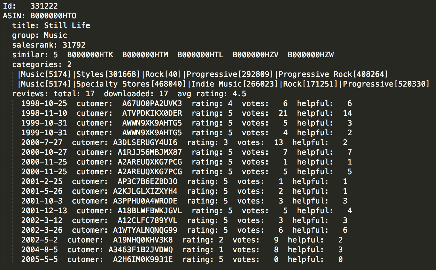
Figure 5
The objective of this section is to create samples of networks to be analyzed. I would be using Hive for the task. I want to see how does the networks of users that have provided one specific rating looks like. To that end, I would create tables of Nodes. There are two types of nodes here Products and Users. In addition, I would extract the edges group by the rating the user have provided. I would extract the data and create the networks using R and Gephi. R would be used to create a file that Gephi can read. The reason to use Gephi is because is easy to do a final filtering of the network to be resented as a graph. Gephi is better in plotting networks.
Figure 6
Creating tables code
Using Hive
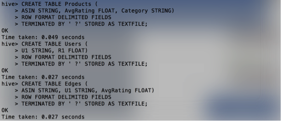
Creating tables
Products table
CREATE TABLE Products (
ASIN STRING, AvgRating FLOAT, Category STRING)
ROW FORMAT DELIMITED FIELDS
TERMINATED BY ‘ ∑’ STORED AS TEXTFILE;
Users table
CREATE TABLE Users (
U1 STRING, R1 FLOAT)
ROW FORMAT DELIMITED FIELDS
TERMINATED BY ‘ ∑’ STORED AS TEXTFILE;
Edge table
CREATE TABLE Edges (
ASIN STRING, U1 STRING, R1 FLOAT)
ROW FORMAT DELIMITED FIELDS
TERMINATED BY ‘ ∑’ STORED AS TEXTFILE;
CREATE TABLE Edges2 (
ASIN STRING, U2 STRING, R2 FLOAT)
ROW FORMAT DELIMITED FIELDS
TERMINATED BY ‘ ∑’ STORED AS TEXTFILE;
CREATE TABLE Edges3 (
ASIN STRING, U3 STRING, R3 FLOAT)
ROW FORMAT DELIMITED FIELDS
TERMINATED BY ‘ ∑’ STORED AS TEXTFILE;
Populating tables code
Populating tables
Products table
LOAD DATA LOCAL INPATH ‘/home/ec2-user/SocialNet/AmaNet.txt’
OVERWRITE INTO TABLE Products;
Products table
LOAD DATA LOCAL INPATH ‘/home/ec2-user/SocialNet/AmaNet.txt’
OVERWRITE INTO TABLE Products;
Users table
LOAD DATA LOCAL INPATH ‘/home/ec2-user/SocialNet/AmaNet.txt’
OVERWRITE INTO TABLE Users;
Edges table
LOAD DATA LOCAL INPATH ‘/home/ec2-user/SocialNet/AmaNet.txt’
OVERWRITE INTO TABLE Edges;
LOAD DATA LOCAL INPATH ‘/home/ec2-user/SocialNet/AmaNet.txt’
OVERWRITE INTO TABLE Edges;
INSERT INTO TABLE Edges5
SELECT ASIN, U2 as U1, AvgRating FROM Edges5;
INSERT INTO TABLE Edges3
SELECT ASIN, U3 AS U1, R3 AS AvgRating FROM Edges3;
Verifying data
SELECT COUNT(*) FROM Products;
SELECT COUNT(*) FROM Users;
SELECT COUNT(*) FROM Edges;
Exporting data
INSERT OVERWRITE DIRECTORY ‘HiveNodesR5’
SELECT ASIN, AvgRating, Category
FROM Products
WHERE AvgRating = 5;
INSERT OVERWRITE DIRECTORY ‘HiveNodesR3’
SELECT ASIN, AvgRating, Category
FROM Products
WHERE AvgRating = 3;
My first visualizations on the previous review were difficult mostly because of the required time to process all the data in a single computer. That made impossible to create so many filters to the data. While a regular computer and python takes some hours to complete the task of reading and filtering, with Hadoop the implementation, requires minutes to run using Hive.
Network Visualizations
The networks are bipartite, the relation is between users and products. Using Hadoop was easy to extract the edges selected by ratings. The filter was made like a relational database compared to the one done in python code where each line has to be read in order to find a lot of points that meets the criteria. Hadoop filters the information as we needed and delivers multiple files, the partition by reducers. Each partition could be considered a sample for network analysis. Taking one of the chunks and the data is loaded into R. Here the graphs are recognized as bipartite setting the attribute “type” to denote which are users and which are products. The following step is to project the user-to-user network.
The network shown in figure 7 is the network of users that have provided ratings of 5 to the products. The color is set as the weighted degree. The darker the color the more weight/connections it has. Even when the network is very dense, there are some nodes that have rated many products. Making the degree higher to other users.
Figure 7
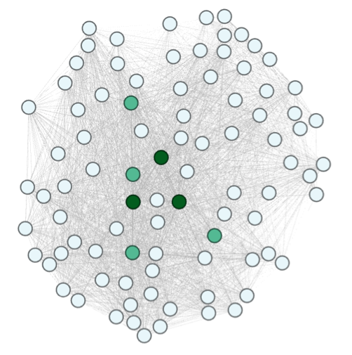
The network below is a network that has provided ratings of 3 to the products. It has been built the same way as the one above. From a bipartite network of products to users, a network of users is projected. This network is even denser that the one of rating five. There may not be many good products, or maybe the users complain more about average products. In any case, there are far more edges. One interesting thing is a group of users that form a local network. This is something that is common to the network that identifies important nodes extracted from the previous analysis(Figure 8). Figure 8 was constructed by snowball sampling.
Figure 8
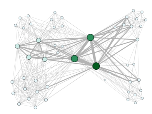
Figure 9
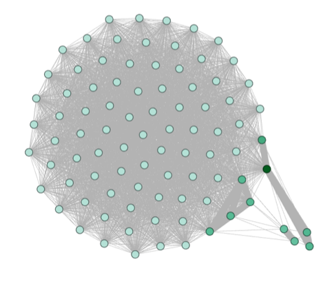
Snowball sampling is done by selecting a node and start walking the edges it has until we get a network of a desirable size. This may produce bias networks. In contrast to the networks created with Hadoop that considers a large amount of data. Nevertheless, the similarity is there. There are some users that tend to read wider types of books. These type of users are the key to create larger networks. Another similarity, that is possible to see in figure 8, is how there are many clusters that are very dense just like the main cluster in figure 9.
Using Hadoop to query large networks provides tools for a more efficient and exhaustive analysis. While in a personal computer I was able to create good samples only by using snowball, with Hadoop I was able to produce more specific filters to the data. The behavior of the networks is evident in a more clear way. For future work joins and more filtering could be performed for a deeper network analysis powered by Hadoop.
HDFS did a good job maintaining the cluster balanced. The column “Use(%)” shown in figures 10 and 11 look very similar. There is more load on the master node as it was also used as a slave while reducing the data, the change in the remaining space was more affected. However, the non-DFS usage is larger too.
Figure 10
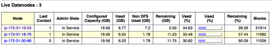
Figure 11

Related


